Stress. Differential equations of equilibrium. Principle of virtual displacements
Stress
Consider a spatially deformable body in a Cartesian coordinate system subjected to a static system of external forces. The system of loading forces is in equilibrium because it also includes reaction forces at the points where the body is fixed. Under the effect of these forces, the body deforms and its initial volume and surface configuration $V_0$, $S_0$ changes to the current configuration $V$, $S$ (Fig. 2.1).
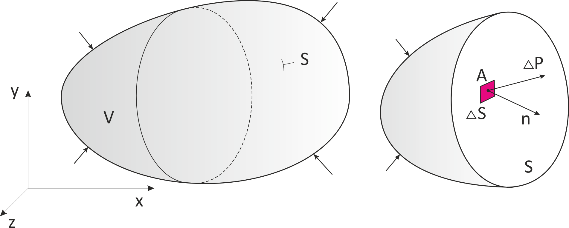
When the body is in equilibrium, every part of it must also be in equilibrium. If we cut the body into two parts with an imaginary plane, it is clear that for these parts to remain in equilibrium, they must act on each other across the imaginary plane with internal forces that ensure their equilibrium. Although, from the six static equilibrium conditions written for the detached part, we can determine the resultants of internal forces at the imaginary plane (which, in elementary elasticity and strength theory, is helpful for solving so-called basic cases of loading of bodies of simple shapes), in the general case, we do not know how the internal forces are distributed over the considered plane; moreover, it is necessary to create a measure to assess the degree of stress on a body at its general point.
If we isolate a very small area around point A in a hypothetical cross-section $\Delta S$, the situation becomes simpler. The internal forces acting on this small area can be averaged and replaced by a resultant force $\Delta \mathbf{P}$ (on a very small area, the moment effect of the internal forces is negligible). As a measure of the stress at this point, the ratio $\Delta \mathbf{P}/\Delta S$ is chosen, which, when the area is reduced to a limit, is known as stress
Stress, expressed as (2.1), is a force vector per unit area; however, it also depends on the direction of the normal of the cross-sectional area (its orthogonal unit vector) because an infinite number of sectional planes can be drawn through point A.
Transformation of stress on the orthogonal planes of the differential element
Assume a special case wherein the cross-sectional planes through point A are parallel to the coordinate planes. In such a case, the stress vectors on the three elementary surfaces $d{{S}_{x}}=dydz$, $d{{S}_{y}}=dxdz$ and $d{{S}_{z}}=dxdy$ (see Fig. 2.2) can be decomposed into components
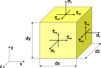
Where ${{\mathbf{e}}_{1}}$, ${{\mathbf{e}}_{2}}$, ${{\mathbf{e}}_{3}}$ are unit vectors in the directions of the coordinate axes, and the nine values ${{\sigma }_{x}}$, ${{\tau }_{xy}}$, ... are the components of the stress vectors on the differential surfaces at a point in the body, as shown in the figure 2.2. The stress components ${{\sigma }_{x}}$, ${{\sigma }_{y}}$, and ${{\sigma }_{z}}$ are known as the normal stresses, and the components ${{\tau }_{xy}},{{\tau }_{yx}},{{\tau }_{xz}},{{\tau }_{zx}},{{\tau }_{yz}},{{\tau }_{zy}}$ are shear stresses. Stress has the properties of a second-order tensor and its components can also be written as a 3x3 matrix with different notation and indexing of its members.
It can be shown that stress is a symmetric tensor
Therefore, in applied mechanics and the FEM, often only six stress components are used, expressed in a column matrix - a (pseudo)vector
Expressing the general stress in its plane using its components
Cauchy’s stress theorem states that by using the stresses in three mutually independent planes passing through point A, it is possible to uniquely express the stress in any arbitrary section plane passing through this point. We express the unit normal vector of such a general section plane as
where $n_x$ , $n_y$, $n_z$ are the direction cosines of the vector in the given coordinate system. Subsequently, the stress in the section plane is the sum of the projections of the stress vectors from the three faces of the element into the direction of vector n
which, using (2.2) gives
and in brief scalar index notation
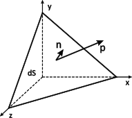
This is the stress that expresses the effect of the removed part of the element on the plane dS (see Fig. 2.3). It is often used when writing the force boundary conditions (for surface pressure or tension) on the surface of a body .
Stress analysis at a point of a body
When analyzing the stress at a point in the body (from the equations of equilibrium of the cut-off part of the element in Fig. 2.3) the relationship (2.7) is used in which the symmetry of the stress tensor is considered, and the following holds
or, in a more illustrative matrix form, only six independent components of stress remain as
By tilting the sectional plane (changing the direction cosines $n_x$, $n_y$, $n_z$) for a given stress vector, we can study the changes in the components of stress $\{\mathbf{p}\}$ and express their values for special types of stress.
Differential Equations of Equilibrium
In continuum mechanics, for the so-called boundary value problem, we know the values (functions) of displacements and loads at the boundary of a body, and we seek the functions for displacements, deformations, and stresses inside the body. In the analytical solution of the problem, we often start from (partial) differential equations of the problem (the sought functions are expressed in terms of gradients of functions), which must be solved with the given boundary and possibly initial conditions. In a loaded body in equilibrium, the stress gradients cannot change independently when moving from point $\text{A}\left( \text{x}\text{,y}\text{,z} \right)\text{ }\!\!~\!\!\text{ }$ to point $\text{A}\left( \text{x+dx}\text{, y+dy}\text{, z+dz} \right)$ they must satisfy the differential conditions of equilibrium. These conditions ensure that even the differential part of the body is in force equilibrium.
From above considerations, it follows that if we select a part of the body in equilibrium with volume V and surface area S, then the integral of stress $\mathbf{p}$ (2.7) over surface S, that is, the resultant of the internal surface forces, must be equal to zero
because this part must also be balanced.
However, body forces $\left\{ \mathbf{b} \right\}={{b}_{i}}\left( x,y,z \right)$ may also act within an object; that is, forces per unit volume, such as the object’s weight, centrifugal force, and magnetic forces, which must also be included in the equilibrium conditions.
By applying Gauss’s divergence theoremsup1, which is used here for three-dimensional space and a tensor quantity, the surface integral in the given relation can be transformed into a volume integral
and because this relationship applies to any volume of the body, the integrand must be equal to zero, leading to scalar differential equations (conditions) for the equilibrium of the body
Considering the symmetry of the stress tensor, this equation can be rewritten as
where we can then use the equations with only six independent stress components
These differential equations must be satisfied by every mechanical stress field within the continuous volume of a body under the given boundary conditions, provided that the equilibrium conditions are satisfied.
In conclusion, the stress considered in this section is the so-called Cauchy (true) stress because it is defined on the deformed (real, current) shape (volume) of the body and acts on the surface defined and created by its current xyz coordinates; this is precisely the measure of stress required for an accurate stiffness and strength assessment of a loaded body. When seeking it from the differential equations or integral variational relations, it becomes necessary to integrate the variables over the unknown deformed volume of the body. Unfortunately, this is associated, especially for nonlinear problems (large displacements, large rotations, large deformations, nonlinear material properties, etc.), with considerable difficulties.
For linear problems, we assume that the effect of differences in the position, shape, and volume of the actual configuration compared to the initial (reference, original) configuration of the body is negligible, and we solve the problem based on the known initial configuration. The stress determined using this configuration is considered to be the Cauchy stress.
Principle of virtual displacements
The principle of virtual displacement (the deformation version of the principle of virtual work) is one of the fundamental starting points for the deformation formulation of the finite element method. It is an integral (energetic) expression of the equilibrium conditions.
We derive the principle of virtual displacements from the differential conditions of the body (2.10). For the sake of simplifying the notation of the intermediate results, we express these in their simplest form
The deformation (displacement) boundary conditions ${{\bar{u}}_{i}}$ are prescribed on the surface of the body ${{S}_{u}}$, and the force conditions (loading) on the surface ${{S}_{p}}$ are in the form of surface traction with components ${{\bar{p}}_{i}}$ (concentrated forces are not considered but may be in the FEM included directly). Subsequently, the differential equilibrium conditions for the body are applied
with essential (Dirichlet) boundary conditions
and natural (Neumann) boundary conditions
where the surfaces of the body $S={{S}_{u}}\cup {{S}_{p}}$, ${{S}_{u}}\cap {{S}_{p}}=0$ and ${{n}_{j}}$ are the components of the unit normal vector to the surface ${{S}_{p}}$. Now, we apply a virtual (imagined, chosen) continuous displacement functions $\delta {{u}_{i}}(x,y,z)$ to the body, which are zero at the points of the given real displacements
Then, for the body according to (2.12), we get
and the integral over the volume of the body must also equal zero Image
Because in (2.16) we can change the functions $\delta {{u}_{i}}$ arbitrarily, this relation holds if and only if the differential equilibrium conditions are satisfied (when the expression in the parentheses equals zero). In this manner, we have obtained another form of expressing the equilibrium conditions for the body.
Using the formula for the derivative of a product ${{\left( {{\sigma }_{ij}}\delta {{u}_{i}} \right)}_{,j}}={{\sigma }_{ij,j}}\delta {{u}_{i}}+{{\sigma }_{ij}}\delta {{u}_{i,j}}$ we can modify (2.12) to
where Gauss's divergence theorem is again used, and the first term in this relation is transformed into a surface integral
which, according to (2.14) and (2.15), changes to
where the components of the virtual displacement on the surface are $\delta u_{i}^{p}$.
Given the symmetry of the stress tensor and the known relationship for the strain tensor ${{\varepsilon }_{ij}}$ [Ch.1], we can write
and we obtain the resulting relation
In matrix notation
The integrands in this relation are scalar values with units of work (Nm); thus, the relation is classified as an energy equilibrium condition. It is a mathematical expression of the principle of virtual displacements, which states that if we apply kinematically admissible virtual displacements to a body in equilibrium, then the virtual work of internal forces is equal to the virtual work of external forces, expressed as
The term virtual work refers to the work performed by real force quantities (stresses and external forces) on virtual displacements. In this imagined experiment, the stresses and external forces does not change; that is, they are independent of the virtual displacements. Additionally, in contrast to the differential equilibrium conditions, the equilibrium conditions for the body (2.19) clearly specify the force boundary conditions.
If the body is divided into a mesh of finite elements, the equilibrium conditions also apply to a finite element, and in the finite element method, the principle of virtual displacements is often used to formulate both linear and nonlinear finite elements.