KINEMATICS OF FINITE (LARGE) DEFORMATIONS

1. Motion of a body. Material and spatial coordinates

In continuum mechanics, a deformable body represents a continuous region of material points (material particles) that generally undergo complex motion in space under loading. This motion can be conceptually divided into the motion of the body as a rigid whole and the deformation caused by changes in the distances between the body’s points. Kinematics studies and describes this motion, regardless of the external and internal forces that cause it. If we do not narrow down this subject matter for our purposes, we would must speak of a continuum rather than a body, of the motion of the particles of the continuum rather than of the body, and we must extend our considerations and relationships to the fields of fluid mechanics and thermomechanics.

Let us call the set of material points constituting the model of a body at time t, its configuration. Let the configuration without deformations at time $t=0$ be the initial configuration of the body. The positions of the material points in the initial configuration will be determined in a Cartesian coordinate system with basis (unit) vectors ${{\mathbf{E}}_{\text{I}}}$ (Fig. 8.1) by the so-called material (Lagrangian) coordinates

In the initial configuration, we denote the material points of the body by capital letters and the other quantities by the index zero: volume ${{V}_{0}}$, area ${{S}_{0}}$, length ${{\ell }_{0}}$, and material density ${{\rho }_{0}}$ .

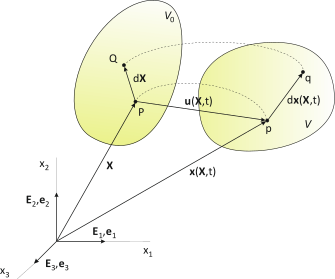
Fig. 8.1

During the loading process, the body deforms and moves in space; at time t, the material points occupy a position given by spatial (Euler) coordinates

where${{x}_{\text{i}}}$are the components of the position vector of a point in the current configuration. The position vectors of points in the current configuration, as can be seen from , can be expressed in a different basis denoted by ${{\mathbf{e}}_{\text{i}}}$; however, we assume that ${{\mathbf{E}}_{\text{I}}}$ and ${{\mathbf{e}}_{\text{i}}}$are identical. For certain quantities, we shall retain their different notations to indicate whether the quantity in question pertains to the initial or current configuration of the body. In the current configuration, we denote the volume as $V$, area as$S$, length as $\ell $ and density as $\rho $ .

We shall now examine the complex physical relationships between the initial and current configurations solely from a kinematic perspective; thus, the function expressing the position of points in the current configuration can be written as

The notation of the motion vector function$\mathbf{x}\left( \mathbf{X},t \right)$ on the right-hand side of this equation is indeed illustrative, but the notation is identical to that of the position vector of a point; therefore, we may also encounter an equivalent notation for the motion of a body in the form

where$\phi \left( \mathbf{X},t \right)$ is a function that describes (maps) the motion.

If we choose the material coordinates$\mathbf{X}$and time t as independent variables, as they appear, for example, in equations and (8.4) – then such a description of motion is called material or Lagrangian, and we refer to it as the Lagrangian (material) formulation. In this case, if we designate an arbitrary material point P in the initial configuration with coordinates ${{\mathbf{X}}_{P}}$, then, in general, the nonlinear function${{\mathbf{x}}_{P}}\left( t \right)=\phi \left( {{\mathbf{X}}_{P}},t \right)$ determines the curved trajectory (path) of material point P (its position vector) during the motion of the body under investigation. For a specific fixed time${{t}_{n}}$, the function$\mathbf{x}=\phi \left( \mathbf{X},{{t}_{n}} \right)$ specifies the deformed configuration of the body at this time.

In the Lagrangian formulation and solution of the problem, we can track the motion and deformation of the body from its initial configuration to its current configuration, which is essential for problems that occur on this path for some reason (e.g., material-related). In addition, it is usually necessary to determine the deformed shape of a body at the end of the motion.

The problem can also be formulated such that the independent variables are $\mathbf{x}$ and t, which is known as the spatial or Eulerian formulation. This description of the motion of continuum particles and the subsequent formulation and solution of the problem are primarily encountered in fluid mechanics. However, independent spatial coordinates are sometimes unavoidable, even in nonlinear structural mechanics problems, where the Lagrangian formulation is preferred, particularly when deriving constitutive equations (the relationship between deformation and stress). Admittedly, the unambiguous link between a physical relationship expressed using one set of coordinates or the other stems from the motion of the body, which is independent of the coordinates. Therefore, it is possible to transform any relationship from one coordinate system to another, although this is not always straightforward.

2. Deformation gradient. Stretch

In the previous section, we showed that if, in the initial (undeformed) configuration, we choose an arbitrary point with position vector$\mathbf{X}$, then its position in the current (deformed) configuration is determined by vector$\mathbf{x}=\phi \left( \mathbf{X},t \right)\equiv \mathbf{x}\left( \mathbf{X},t \right)$. The non-linear vector function$\phi $ can be expanded into a reduced Taylor series (linearised in the neighbourhood of the point$\mathbf{x}$) for a fixed time t

where the expression

is the strain gradient. As it is the gradient of a vector function, it is a second-order tensor

During the deformation of a body, the line segment$d\mathbf{X}$ connecting two neighbouring material points$\mathbf{X}$ and$\mathbf{X}+d\mathbf{X}$ is displaced and transformed into the line segment$d\mathbf{x}$ (Fig. 1), whereby the following holds

The strain gradient along contains important information about the deformation (stretching and rotation) of the material line segment $d\mathbf{X}$ following its deformation transformation to $d\mathbf{x}$; this is, in fact, information regarding the deformation in the vicinity of the point defined in the initial configuration by vector$\mathbf{X}$. The spatial displacement (movement) of this point is determined by the displacement vector $\mathbf{u}\left( \mathbf{X},t \right)=\mathbf{x}\left( \mathbf{X},t \right)-\mathbf{X}$ (see Fig. 8.1), and for the deformation of the line segment$d\mathbf{X}$ the following also holds

where $\mathbf{I}$ is the unit tensor, and $\mathbf{D}$ is the displacement-derivative tensor or displacement gradient tensor.

For the algorithmization and any subsequent programming, as well as for greater clarity, it is useful to express the important tensors in matrix form. The deformation gradient, denoted by , is

and the matrix of the displacement-derivative tensor given by (8.9)

It follows from (8.9) the relationship

which, in FEM, is the fundamental basis for determining the strain gradient at the integration points of the elements in the computational model of the body. In the iterative process, we can express, in the finite elements, the approximate functions of the displacement components $\mathbf{u}\left( X,Y,Z,t \right)$ and, from these, the necessary derivatives into . From the FEM perspective, tensors $\mathbf{D}$ and $\mathbf{F}$ can be treated as known quantities in the subsequent analysis of deformation kinematics.

3. Measures of deformation

Let us consider, in the initial configuration of the body, a line element $d\mathbf{X}$ of length $dL$, which, under the effect of the body’s deformational motion, stretches (or shortens) to $d\mathbf{x}$ of length$d\ell $ and, in general, rotates. According to (3.9) , the following holds

Dividing both sides of this equation by the product$dLd\ell $, we obtain

where

are unit vectors that determine the directions of the line element before and after deformation, respectively. The stretch ratio $\lambda $ determines the relative change in length of the element

We modify the equation (8.14) by taking the scalar product of the vectors with themselves on both sides

and, through successive simplification, we obtain

where, as can be seen, the following holds for the so-called right Cauchy–Green deformation tensor

Thus, we obtained a useful measure of the deformation of a body subjected to spatial stress. If, in the initial (reference) configuration, we specify the direction $\mathbf{N}$ for the line element $d\mathbf{X}$, the tensor$\mathbf{C}$ allows us to determine the elongation $\lambda $ of this element following its deformation to $d\mathbf{x}$ in the current configuration.

An important and frequently used strain tensor is obtained from an analogous analysis of the difference of the squares of the lengths$d\ell $ and $dL$

where

is the Green–Lagrange deformation tensor. By utilising the inverse relationship (8.9) and following a similar procedure (but now eliminating $\mathbf{X}$), we would obtain the Almansi (Eulerian) deformation tensor, which is a function of the spatial coordinates

where

is the left Cauchy–Green deformation tensor.

Since we are interested in the deformation of a body, we shall focus primarily on Lagrangian measures, which are functions of material coordinates, and in particular on the Green–Lagrangian deformation tensor $\mathbf{E}$. Its main properties are summarized as follows:

• It is a symmetric tensor and its independent components can be expressed in pseudovector form (suitable for matrix operations and computer processing) after expansion according to the relations (8.20) and (8.12)

• It can be shown that it is independent of the pure rotation of the body as a rigid body, which is a natural requirement for a deformation measure. Consider an undeformed body in its initial configuration, which moves as a rigid body. Such a motion can be decomposed into a rotation about the origin of the coordinate system and a purely translational motion

Where $\mathbf{R}$ is the rotation tensor, and ${{\mathbf{x}}_{T}}$ is a translation vector. In this case, however, according to (8.9), the following holds: $\mathbf{F}=\mathbf{R}$ and no deformation occurs, because from the definition of the Green–Lagrange deformation tensor we obtain

where it has been taken into account that $\mathbf{R}$ is an orthogonal tensor.

• It is a generalization of the uniaxial Green’s strain ${{\varepsilon }_{G}}=\tfrac{1}{2}({{\lambda }^{2}}-1)$ , which we obtain from it in the case of pure uniaxial deformation. In that case, the strain gradient according to (8.10) is

and from (8.20) we obtain

For general deformation, according to (8.19), the following holds

and after dividing by $d{{L}^{2}}$

where ${\mathbf{N}=d\mathbf{X}}/{dL}\;$ specifies the chosen (specified) direction of elementary segment d$\mathbf{X}$ originating from the point$\mathbf{X}$ in the initial configuration of the body.

Thus, for an elementary line segment transformed into the current configuration $d\mathbf{x}=\mathbf{F}d\mathbf{X}$, it is possible to determine the Green’s deformation from $\mathbf{F}$ and, using (8.14) or (8.15) , its direction $\mathbf{n}$.

Example 8.1: Deformation analysis using the deformation gradient

A planar square material particle with very small (theoretically infinitely small) unit dimensions, positioned for simplicity at the origin of the coordinate system as shown in the figure underwent a deformation movement to a steady-state position according to the function

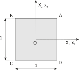
Fig. 8.2

According to these equations, the centre of the particle O(0,0) has moved to the position o(3,1), which we can regard as the displacement of the particle, and the corner point A(0.5; 0.5) to the position

By analogy, we would also obtain the new positions of the other corner points: b(1.65,0.70), c(2.85,-1.30), d(4.35,1.30). In Fig. 8.3, we plotted these points to scale and connected them, providing an illustration of the new position and deformation of the particle. The deformation gradient of this transformation is

The strain gradient enables the analysis of the strain in the immediate vicinity of a point whose position in the initial configuration is given by vector$\mathbf{X}$. Let us consider, in the initial configuration of the body, a line element

of length$dL=1/\sqrt{2}=0.7071$ , as shown in Fig. 8.3.

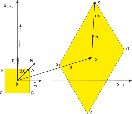
Fig. 8.3

According to (8.13), the following applies to deformation:

This vector is represented by a dotted line in Fig. 8.3, and its actual position is determined by the displacement (see also Fig. 8.1). The following applies to the length (absolute magnitude):

The stretch factor is

The unit vector $\mathbf{n}$, indicating direction$d\mathbf{x}$, can be determined from (8.14) or from (8.15)

4. Polar decomposition of the strain gradient

Based on Cauchy’s theorem on the polar decomposition of a tensor, the strain gradient can be decomposed in two ways into the product of two tensors

where the symmetric tensors $\mathbf{U}$ and $\mathbf{V}$ are the right and left strain tensors (named according to their position relative to $\mathbf{R}$), respectively, and $\mathbf{R}$ is the orthogonal rotation tensor (${{\mathbf{R}}^{-1}}={{\mathbf{R}}^{T}}$). For the right Cauchy–Green deformation tensor, the following then holds

where symmetry $\mathbf{U}$ (${{\mathbf{U}}^{T}}=\mathbf{U}$ ) and orthogonality $\mathbf{R}$ are utilized.

The Green–Lagrange deformation tensor is

The deformation relation for$d\mathbf{X}$ (3.13) can be written as

where the auxiliary brackets indicate that the deformation $d\mathbf{X}$ occurs in two steps: first, $d\mathbf{X}$ is stretched to$d\mathbf{{X}'}=\mathbf{U}d\mathbf{X}$ and then rotated to the $d\mathbf{x}=\mathbf{R}d\mathbf{{X}'}$. Therefore, the deformation motion of a material particle consists of three separable phases: translation, stretching, and rotation phases.

The problem that needs to be addressed when decomposing the deformation gradient is the determination of the tensor $\mathbf{U}$, since $\mathbf{R}$ is then calculated from the relation

To ensure that the strain gradient is decomposed into pure stretching and pure rotation, the line elements$d\mathbf{X}$ and $d\mathbf{{X}'}$ in must be parallel, from which it follows that

and furthermore, since according to $d\mathbf{X}=\mathbf{N}dL$

The equation represents a linear eigenvalue problem, the solution of which consists of the principal stretches${{\lambda }_{K}}$ and associated principal directions ${{\mathbf{N}}_{K}}$ of tensor $\mathbf{U}$. The unit vectors ${{\mathbf{N}}_{K}}$, due to symmetry $\mathbf{U}$, form an orthonormal basis for the spectral representation (spectral decomposition) of $\mathbf{U}$, and the following holds

We shall write this important relationship in matrix form

Since raising $\mathbf{U}$ to a natural number does not change the basis, (8.35) is a special case of the general relation

Using (8.37), the Cauchy–Green deformation tensor (8.29) can be expressed as

and for the Green–Lagrange deformation tensor, according to (8.30), we obtain

The important logarithmic deformation tensor can be determined from (8.37) as a special case for $n=0$

From a comparison of (8.35) and (8.37) , it follows that (8.34) can be rewritten as

and since ${{\mathbf{U}}^{2}}={{\mathbf{F}}^{T}}\mathbf{F}$, the values${{\lambda }_{K}}$ and ${{\mathbf{N}}_{K}}$ are determined using the standard procedure for solving the eigenvalue problem (8.41) from the equations

and from the conditions for their non-zero roots

Using the known values${{\lambda }_{K}}$ and ${{\mathbf{N}}_{K}}$, the tensor $\mathbf{U}$ is determined using (8.35) or alternatively using (8.36) .

Example 8.2   Polar decomposition of the strain gradient in a plane problem

We need to determine the matrices $\mathbf{U}$ and $\mathbf{R}$ of the deformation gradient from Example 8.1

From (8.29) , we obtain

From (8.42) , we obtain a system of homogeneous equations which has a non-zero solution only if the determinant of the matrix of its coefficients, (8.43) , is equal to zero

Solving this quadratic equation yields $\lambda _{1}^{2}$ ,$\lambda _{2}^{2}$ , and, after taking the square root of the principal strain ratios, we obtain ${{\lambda }_{1}}=3.3264$ and${{\lambda }_{2}}=1.8398$ . We determine the unit vectors of the principal directions from (8.42) by successively substituting ${{\lambda }_{1}}$ and ${{\lambda }_{2}}$ and calculating the terms ${{\mathbf{N}}_{1}}$ and ${{\mathbf{N}}_{2}}$ from these equations

The direction of the first principal strain${{\lambda }_{1}}$ was obtained from the vector ${{\mathbf{N}}_{1}}$: $\cos {{\varphi }_{1}}=0,8558$ and $\sin {{\varphi }_{1}}$ 0 $\to $ ${{\varphi }_{1}}={{31,15}^{\circ }}$. The principal directions are mutually orthogonal; thus, the angle ${{\varphi }_{2}}={{121,15}^{\circ }}$ (Fig. 8.4).

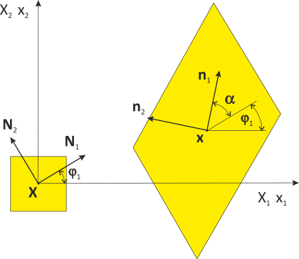
Fig. 8.4

The stretch matrix, according to (8.36) , is

and the rotation matrix is obtained from (8.32)

Since the rotation matrix for a vector in a plane by an angle $\alpha $ is

it is easy to see that the directions of the principal strains (unit vectors ${{\mathbf{N}}_{i}}$) rotate by an angle$\alpha ={{47,35}^{\circ }}$ when a load is applied to the particle.

Based on this analysis, it can be concluded that the particle stretches in the direction given by the angle ${{\varphi }_{1}}={{31,15}^{\circ }}$ by a value of ${{\lambda }_{1}}=3,3264$ , in the perpendicular direction by a value given by ${{\lambda }_{2}}=1,8398$. Then having been deformed in this way, it rotates as a rigid body by an angle of $\alpha ={{47,35}^{\circ }}$ (see Fig. 8.4).

By formalizing this procedure into an algorithm (in FEM, combined with geometric and temporal discretization), it is possible to determine the deformation tensors (matrices) (8.38) to (8.40) and possibly others, which, as functions of $\mathbf{X}$ and t, define the deformation motion of the body.

5. Change in volume

The deformation of a body causes a change in its volume and a consequent change in the density of the material. Just as the deformation changes at every point in the body, so too do the volume and density; these changes must be examined and expressed in terms of the differential volume of a material particle in the body.

In the initial configuration of the body, consider a volume element $d{{V}_{0}}$ whose edges are parallel to the coordinate axes and are given by the vectors $d{{\mathbf{X}}_{1}}=d{{X}_{1}}{{\mathbf{E}}_{1}}$ ,$d{{\mathbf{X}}_{2}}=d{{X}_{2}}{{\mathbf{E}}_{2}}$ and$d{{\mathbf{X}}_{3}}=d{{X}_{3}}{{\mathbf{E}}_{3}}$, where ${{\mathbf{E}}_{1}}$ ,${{\mathbf{E}}_{2}}$ and ${{\mathbf{E}}_{3}}$ are unit orthogonal vectors (Fig. 8.5).

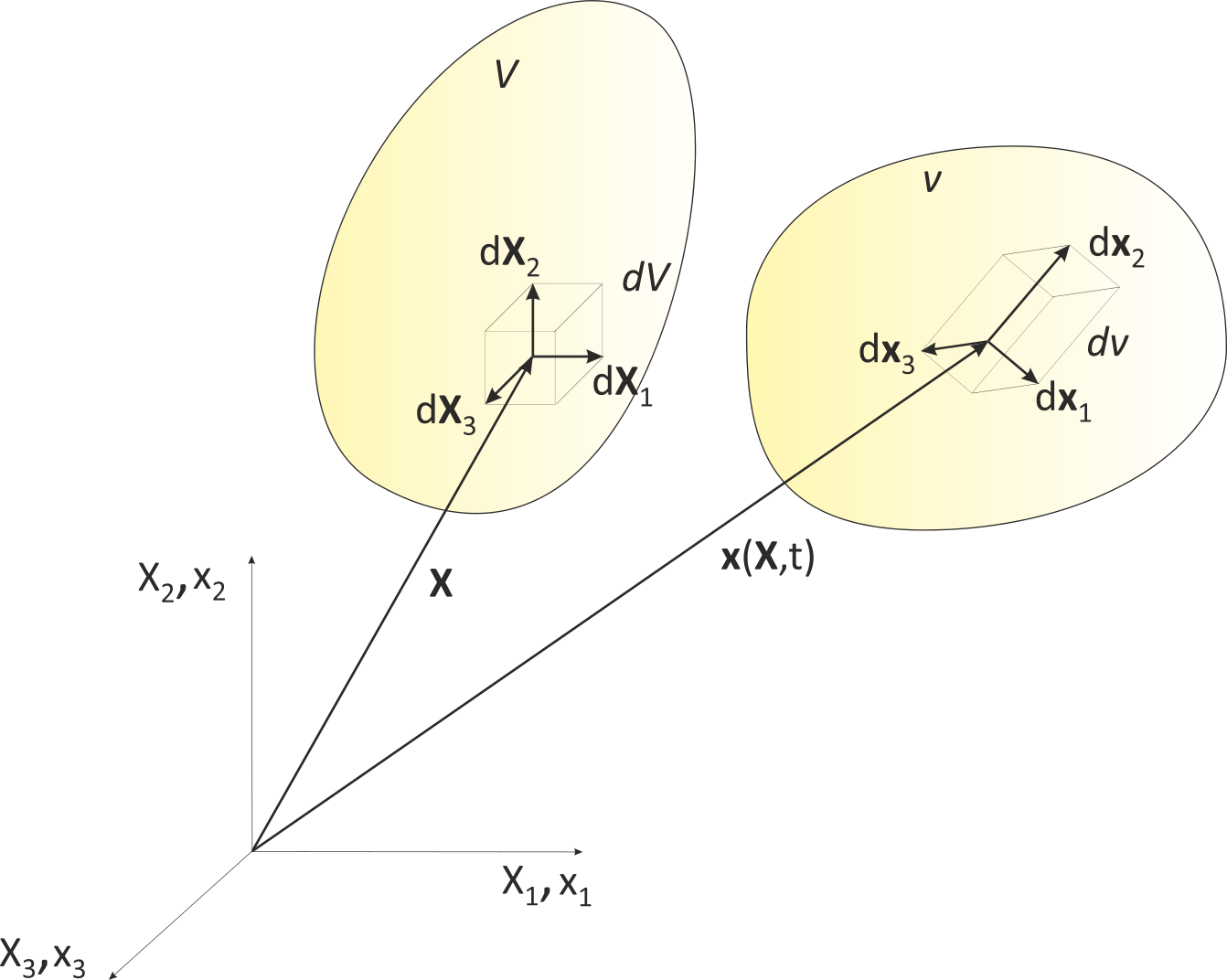
Fig. 8.5

The volume of this element is

As we know from the previous section, the motion of the element can be composed of three phases: its translation to the position $\mathbf{x}=\mathbf{x}(\mathbf{X},t)$ without any change to its vectors or volume, followed by the stretching of its vectors according to the relation (8.13)

associated with a change in the element volume, and finally, its rotation without any change in volume. The deformed element will again be a hexahedron with three parallel pairs of faces (Fig. 8.5), whose edge vectors will be

From vector analysis, we know that the volume of a hexahedron defined by the vectors of its edges is the scalar triple product of these vectors; therefore, the changed volume of the element is

If we recall the deformation gradient (8.10)

we see that the vectors ${\partial \mathbf{x}}/{\partial {{X}_{i}}}\;$ in (8.49) are in fact columns of the strain gradient, and their triple product is the determinant (Jacobian J) of the tensor $\mathbf{F}$.

Then, the following also holds for the modified volume of the element

During deformation, the mass of the body remains unchanged; therefore, the masses of the elements must also be conserved, and the following equation is applicable:

The law of conservation of mass (the continuity equation) then takes the form

It follows from (8.50) that

because the volume of the deformed element cannot be zero or negative.

Example 3: Calculation of the volume of a deformed material element

A cubic material particle with very small (theoretically infinitely small) unit dimensions (Fig.8.6) is subjected to plane deformation in the plane${{X}_{1}}{{X}_{2}}$ (the dimension in the direction${{X}_{3}}$ does not change).

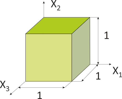
Fig. 8.6

Its deformation gradient in the current loading step is

The initial volume of the element is unit volume $dV=d{{X}_{1}}d{{X}_{2}}d{{X}_{3}}=1$ and for its deformed volume along (8.49) , the following applies

or alternatively, according to (3.50)

The volume of the element after deformation was 6.12 times greater than that before deformation (Fig. 8.4).

6. Change in area

When transforming a surface load between the initial and current configurations, it is necessary to know the relationship between the surface element vector in the initial configuration

and its value after deformation (Fig. 8.7)

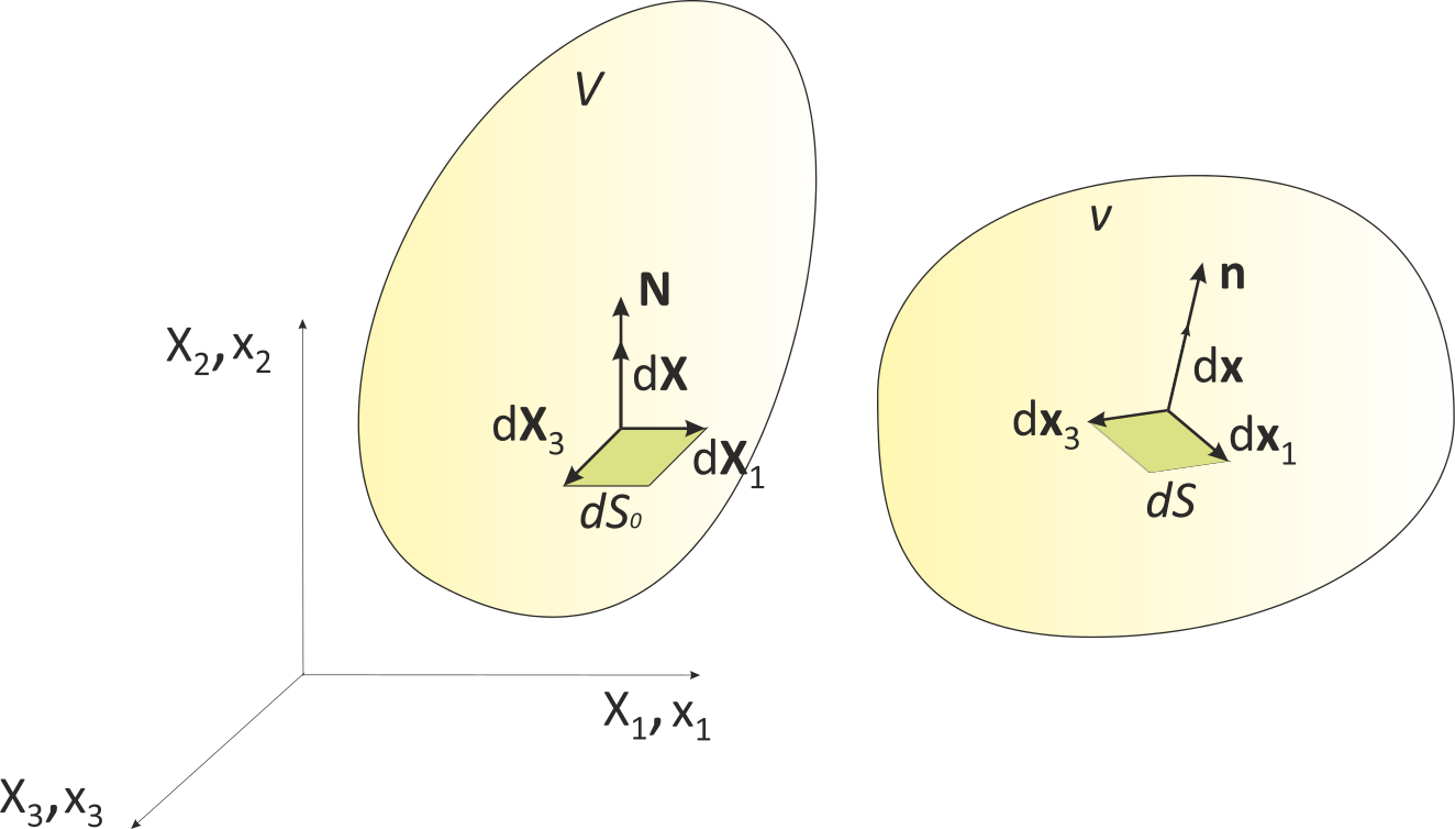
Fig. 8.7

where N and n are unit normal vectors. Let us choose a line element $d\mathbf{X}$ such that $\mathbf{N}\cdot d\mathbf{X}>\text{0}$ and define the volume $d{{V}_{0}}$from the vectors $d{{\mathbf{X}}_{1}},\ d{{\mathbf{X}}_{3}}\ and\ d\mathbf{X}$ and the volume $dV$ from the vectors$d{{\mathbf{x}}_{1}},\ d{{\mathbf{x}}_{3}}\ \text{and}\ \ d\mathbf{x}=Fd\mathbf{X}$ . Then, according to (8.49), the following holds for the deformed volume of such an element

The volume of the deformed element can also be expressed in terms of

By comparing the right-hand sides of these equations, we obtain

and from this, the so-called Nanson’s formula

The absolute value of the area in the current configuration, using the values from the initial configuration, is obtained by scalar-multiplying the vectors on both sides of the first of these equations by themselves, taking the square root, and adjusting using the relations for the right-hand and left-hand Cauchy–Green deformation tensors