Beam instability and stress stiffening
Interesting insights can be obtained by analyzing the effect of the geometric stiffness matrix on the overall stiffness of an element. For this purpose, we express the stiffness matrix of the beam finite element (see in femapplied.com "Slender plane beam element for large displacements and rotations") at its special position, as shown in Fig. 6.1.
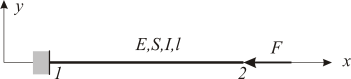
Fig. 6. 1
The axis of the element is identical to the global axis x ($\sin \beta =0$,$\cos \beta =1$), the element is without bending load (${{\mathbf{K}}_{GM}}=\mathbf{0}$), and the pressure axial force was chosen to demonstrate the loss of stability of the beam. The material and geometric matrices of such an element are determined from (5.19) using the simple Mathematics 7 program shown in Fig. 6.2. As can be assumed, based on what we have discussed about this matrix, the material stiffness matrix is identical to the linear stiffness matrix of the element expressed in the local coordinate system.
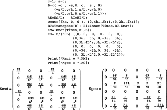
Fig. 6. 2
The global stiffness matrix of a single-element body rigidly fixed in node 1 and loaded by a compressive force F (Fig. 6.1) is obtained by omitting the first three rows and columns in both matrices, as they correspond to the removed (zero) degrees of freedom.
A comparison of the matrix members in (6.1) shows a well-known knowledge of the technical practice: the compressive axial force of the beam decreases its transverse (bending) stiffness (decreases the absolute values of the members of the resulting matrix), and vice versa. In the first case, we are talking about stress softening, in the second about stress stiffening. This is only relevant for slender (thin) structural members with low bending stiffness (slender beams and rods, cables, thin plates, and shells) because, in other cases, the ${{\mathbf{K}}_{M}}$matrix members are negligibly small compared to the ${{\mathbf{K}}_{M}}$members.
In general, the members of a geometric matrix are functions of the axial or membrane stress (in our simple example $\text{N} = \sigma {{\text{S}}_{\text{0}}} = \text{-F}$) and therefore the geometric stiffness matrix is often called the stress stiffness matrix, or, in connection with the iterative process, the initial stress stiffness matrix, since the stress value known at the beginning of the step must be considered in the iteration step.
Because the geometrical stiffness matrix depends to a large extent only on the magnitude of the stress, its influence on the stiffness of the slender body can be significant even for small displacement and rotation problems. Two typical examples of such situations that need to be recognized in terms of the calculation procedure are illustrated by the beams in Fig. 6.3.
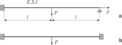
Fig. 6. 3
In the first case, a prestressed beam with a known prestressing force F independent of force P. A classical linear FEM program, which does not have a built-in geometric matrix calculation, would solve this problem without affecting the force F on deflection. With a significant amount of force F, unrealistic results are obtained. The same applies to the second example where the rigid constraints of the beam do not allow the axial movement of its ends, which causes a tensile force with a prestressing effect on the lateral deflection.
From a computational perspective, these geometrically nonlinear problems differ from each other in the following manner: in the first case, the axial force and, hence, the geometric matrix are known, and the calculation can be performed without an iterative process; in the latter case, an iterative process is necessary to calculate the final values of the axial force and geometric matrix.
The need to consider stress stiffness is quite common in computational practice because it occurs in quasi-linear and nonlinear problems not only at static but also at dynamic loading (altered or varying stiffness affects the dynamic properties of the body) and is induced not only by mechanical loads but also by other types of loads, such as temperature load, initial and residual stresses in the material, etc.). The basic calculation procedures that consider the stress stiffness are shown in the ANSYS Mechanical APDL calculations of simple beams in Fig. 6.3, however, the procedures are the same for complex real problems of this type.
Example 6.1
Consider the beam shown in Fig. 6.3a. Assume that P = 100 N, F = 1000 N, $\ell $= 1 m, E =2 1011 Pa,
$\upsilon $= 0.3, $\rho $ = 7850 kg / m3; The cross-section is a square with an area A = 1 cm2. Calculate:
a) Maximum deflection of beam first without prestressing force F and then with it.
b) The first natural vibration frequency of the beam without prestressing by force F and then with it.
c) Modify the beam as shown in Fig. 6.3b and determine the maximum deformation.
The problem can be calculated in the interactive mode of the ANSYS Mechanical APDL program using the following commands:
Utility Menu>File>Change Jobname... /FILNAM = Buckling;
Preprocessor>Element Type>Add/Edit/Delete, Add, Beam, 2 node 188, OK, Close;
Preprocessor>Sections>Beam> Common Sections, B = 0.01, H = 0.01, OK;
Preprocessor>Material Props>Material Models, Favorites, Linear Static, Density, DENS = 7850, OK, Linear Isotropic, EX = 2e11, PRXY = 0.3, OK, Material, Exit;
Plot Controls> Symbols, All Aplied BCs, OK;
Preprocessor>Modeling>Create>Keypoints>In Active CS... X = 0, Y = 0, Apply, X = 1, Y = 0, Apply, X = 2, Y = 0, OK;
Preprocessor>Modeling>Create>Lines>Lines>Straight Line, Click: KP1, KP2, KP3, OK;
Preprocessor>Meshing>Mesh Tool... Lines, Set, Pick All, Ndiv = 10, OK, Mesh, Pick All, Close;
Main Menu>Solution>Define Loads>Apply>Structural>Displacement>On Keypoints, Click KP1, OK, All DOF, Apply, Click KP3, OK, UY, UZ, ROTX, ROTY, OK;
Main Menu>Solution>Define Loads>Apply>Structural>Force/Moment>On Keypoints↑ P: KP2, OK, FY = -100, Apply, Click KP3, OK, FX = 1000, OK;
SAVE_DB;
Solution>Analysis Type>New Analysis, Static, OK;
Solution> Analysis Type>Sol'n Controls, Calculate prestress effects = ON, OK;
Solution> Solve> Current LS, OK;
ANSYS Main Menu> General Postproc> Plot Results>DeformedShape>Def+undeformed, OK;

Solution>Analysis Type>New Analysis..., Modal, OK;
Solution>Analysis Type>Analysis Options..., No. of modes to extract = 1, No. of modes to expand = 1, PSTRES= ON, OK, OK;
Solution> Solve> Current LS, OK;
General Postproc>Results Summary;
Result: Freq = 13.08 Hz
Solution>Analysis Type>Analysis options, Incl prestress effects? = No, OK, OK;
Solution> Solve> Current LS, OK;
General Postproc>Results Summary,
Result: Freq = 8.98 Hz
Solution>Analysis Type>New Analysis>Static, OK;
Solution>Sol'Controls>Analysis Option, Large Displacement Static, Time at end of load step = 1, Number of substeps = 5, Max. no. of substeps = 10, Min. no of substeps = 1, OK;
Solve, Current LS, OK;
General Postproc> Plot Results>DeformedShape, Def +undeformed, OK;

Solution>Define Loads>Delete>Structural>Force/Moment>On Keypoints↑ P, KP3, FX, OK;
Solution>Define Loads>Apply>Structural>Displacement>On Keypoints↑ P: KP1, KP3, OK, All DOF, OK;
Solution>Analysis Type>New Analysis..., Static, OK;
Solution>Analysis Type>Sol'Controls..., Large Displacement Static, Time at end of load step = 1, Number of substeps = 20, Max no. of substeps = 20, Min no. of substeps = 10, OK;
Solution>Solve>Current LS, OK;
General Postproc>Plot Results>Deformed Shape, OK;
The program will plot the deflection curve of the beam and display the maximum deflection DMX = 0.01226 m
Ansys Toolbar>Quit>Save Geom+Loads, OK;
The calculation showed the importance of considering the prestressing effects for problems of this type: the maximum deflection without the prestressing effect (linear calculation) was 44.52 mm, and the prestressing force F reduced it to 21.18 mm. The prestressing also increased the transverse (bending) stiffness of the beam and increased the first natural frequency of the beam from 8.98 to 13.08 Hz.
Now, returning to the beam element in Fig. 6.1. The element is fixed on one side and loaded with a compressive force F on the other. Its stiffness matrix is expressed in (6.1) as the sum of the material and geometric stiffness matrices. It can be observed that as the absolute magnitude of force F increases, the diagonal term of matrix K may be zero and the matrix will be singular. We have already mentioned such a situation in the previous sections, and we call such a state of the body the bifurcation point, equilibrium split point, or stability-loss point. The load causes this condition is called the critical load.
A matrix is singular when its determinant equals zero; therefore the critical value of force F in (6.1) is calculated from the condition det K = 0. For simplicity of calculation we use unit values of the problem parameters and the condition is
For the calculation we use a simple Mathematica program. We got $F_{crit} = 2.486\ \text{N}$. The critical (buckling, Euler) force for such a case of the beam is
The above procedure for calculating the critical load value for a structure with a tendency to lose stability can be generalized and is called linearized buckling. At this problem the FEM program solves the generalized problem of eigenvalues
where ${\lambda}_{crit}$ is the critical load factor of the structure, and vector ${\phi}_{crit}$ contains the normalized displacement amplitudes of the structure model nodes after the loss of stability. This is analogous to the calculation of the natural frequencies and eigenmodes of the body; however, only the first eigenvalue and first eigenmode have physical meaning. Although the calculation is simple, it has some limitations:
1. The stiffness matrices determined for the undeformed body position were used in the calculation; therefore, the results are reliable only for situations in which the assumptions of the linear problem are not violated before the critical state (there are no significant displacements, rotations, and deformations).
2. Under loading, the assumption of a linear increase in all loads and stresses proportional to the multiplier $\lambda $ is valid.
3. There are no significant geometrical, load and material imperfections on the body
4. It is not necessary to determine what happens to the body after loss of stability
If these conditions are not met, the stability problem must be solved geometrically, possibly as a physically nonlinear problem. However, in terms of their validity, linearized buckling provides usable results that are practically identical to those of iterative nonlinear calculations. If the effect of self-weight can be neglected, the buckling of straight rods, beams, and loss of stability of rotationally symmetrical shells and bodies are typical cases where linearized buckling can be used.
In the case of real structures, the conditions for linearized buckling are usually not fulfilled; therefore, it is recommended to calculate the loss of stability limit load using a nonlinear strength calculation. It is a static non-linear FEM calculation with a gradually increasing load up to a state where the body collapses or a sharp transition to another (equilibrium) state, manifested by either divergence or a strong instability of the iterative procedure. The results are then judged using a suitable graphical or numerical postprocessor. The great advantage of such a procedure is the possibility of incorporating and considering the effect (assumed, estimated) imperfections, which always exist in real structures (pressure forces outside the neutral cross-sectional axis, failure to make the ideal shape, material inhomogeneities and cracks, the possibility of weakening the strength by local exceedance of the yield limit, significant changes in geometry during loading, etc.). The mechanism of structural stability loss due to imperfections can differ significantly from that of the idealized linearized calculation..
Consider the steel beam in Fig. 6.1 with values $L$ = 2000 mm, E = 200000 MPa and a circular cross-section with I = 1000 mm4. In an ideal state, under the load of compressive force F and neglecting its own weight, the critical buckling force is
If the force F acts outside the center of gravity of the cross-section with eccentricity e, the relationship between the force and the maximum deflection (at the free end of the beam) can be determined according to the relations for the bending-buckling combination [1]
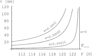
Fig. 6. 4
where $k=\sqrt{{F}/{EI}\;}$. The dependence is shown in Fig. 6.4 We can see the difference from the ideal state (e = 0), which is the result of the linearized calculation. The bifurcation point disappears, the beam can acquire unacceptably large deflections even before reaching the critical force value. This is a simple illustration that, with the exceptions mentioned above, real structures need to be checked using nonlinear analysis.
In the following two examples, we show the computational procedure for solving the loss of stability in ANSYS. Both bodies are without imperfections, and for comparison, we solve them using both procedures. In the first example, the body fulfilled the conditions for linearized calculation, whereas in the second example, the body violated these conditions by precluding the actual collapse of the body through significant movements and rotations of the body.
Example 6.2
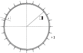
For a planar ring with a square cross-section and $a\times a$ in the figure, determine the critical value of the continuous load q first by using a linearized buckling and then by a non-linear calculation. The ring can only deform in its plane and we assume the linear elastic properties of the material under load. It is given: R = 0.5 m, a = 1 cm, E = 2 E11 Pa.
Theoretical solution gives
Utility Menu>File>Change Jobname... /FILNAM = RING;
Preprocessor>Element Type>Add/Edit/Delete, Add... Beam 3node 189, OK, Close;
Preprocessor>Sections>Beam>Common Sections... Sub-Type: B = 0.01, H = 0.01, OK;
Preprocessor>Material Props>Material Models... Favorites, Linear Static, Linear Isotropic, EX = 2e11, PRXY = 0.3, OK, Material, Exit;
Preprocessor>Modeling>Create>Lines>Arcs>Full Circle, Global Cartesian: 0, 0, 0, OK, 0.5, OK;
Preprocessor>Modeling>Create>Keypoints>In Active CS, OK;
Preprocessor>Meshing>Mesh Attributes>All Lines... Pick Orientation Keypoint = Yes, OK, Click: KP5 (the center of the circle), OK;
Preprocessor>Meshing>Mesh Tool, Lines, Set, Pick All, NDIV = 8, OK, Mesh, Pick All;
Solution>Define Loads>Apply>Structural>Displacement>On Keypoints, Click: Top and bottom point , OK, Mark UX, Apply, Click: Left and right point, OK, Mark (only) UY, Apply, Click all 4 points of the circle, OK, Mark UZ, ROTX, ROTY, KEXPAND = Yes, OK;
Save_DB;
Solution>Define Loads>Apply>Structural>Pressure>On Beams, Pick All, VALI = -1, OK;
Solution>Analysis Type>Sol’Controls... Calculate prestress effects = ON, OK;
Solution> Solve> Current LS, OK, Finish;
Solution>Analysis Type>New Analysis... Eigen Buckling = ON, OK;
Solution>Analysis Type>Analysis Options... NMODE = 1, OK;
Solution> Solve> Current LS, OK;
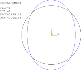
General Postproc>Results Summary...: ${{\lambda }_{krit}}$ = 3998.4
ANSYS Main Menu> General Postproc> Read Results... Last Set;
ANSYS Main Menu> General Postproc> Plot Results>Deformed Shape... Def +undeformed, ON, OK;
Solution>Analysis Type>New Analysis... STATIC, OK;
Solution>Analysis Type>Sol’n Controls... Large Displacement Static, Time at end of substep = 1.0, Number of substeps = 150, Automatic time stepping = OFF, Frequency: Write every substep, OK;
Solution>Define>Loads>Apply>Structural>Pressure>On Beams, Pick All, VALI = -5000, OK;
Solution>Define>Loads>Apply>Structural>Force/Moment>On Keypoints ↑ Click the left point of the circlee, OK, Lab = Fx, VALUE = 10, OK;
Solution> Solve>Current LS, OK;
General Postproc>Read Results>Last Set;
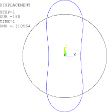
General Postproc>Plot Results>Deformed Shape... Def + undeformed, ON, OK;
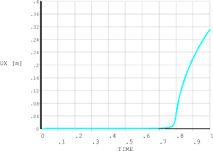
TimeHist Postpro>Variable Viewer... Click the first icon from left, Nodal Solution, DOF Solution, X-Component of displacement, OK, Click the Circle left point, OK, Click the third icon from left;
Ansys Toolbar>Quit>Save Geom+Loads, OK;
The linearized calculation yielded a critical pressure value of ${{q}_{crit}}$= 3998.4 N/m, which was practically identical to the theoretical solution. The value of the critical pressure in a nonlinear solution can be obtained from the above graph of the dependence of the increasing load and vertical displacement of the upper point of the central circle of the ring. A sharp displacement increase occurred at the value of ${{q}_{crit}}\approx 0,8\cdot 5000=4000$Pa. A more accurate view of the critical point can be obtained by displaying a graph at itervals of 0.75 to 0.85 times the load time. The use of linear buckling is, as can be seen, justified in this case.
In a nonlinear calculation, the ideal rotationally symmetrical problem must be disrupted by a small force or deformation imperfection to obtain a smal bend.
Example 6.3
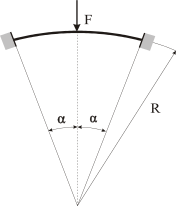
For a curved planar beam (arc) in the figure with a square cross-section $a\times a$, determine the critical value of force F by first calculating the linearized buckling and then performing a non-linear calculation. The beam can deform only in its plane and we assume linear elastic properties of the material under load. It is given: R = 1 m, a = 4 mm, E = 2 E11 Pa, $\alpha ={{20}^{\circ }}$.
Perform the non-linear calculation by the arc-length method.
Utility Menu>File>Change Jobname, /FILNAM = ARC;
Preprocessor>Element Type>Add/Edit/Delete, Add, Beam 3node 189, OK, Close;
Preprocessor>Material Props>Material Models, Favorites, Linear Static, Linear Isotropic, EX = 2e11, PRXY = 0.3, OK, Material, Exit;
Preprocessor>Sections>Beam>Common Sections... Sub-Type: B = 0.004, H = 0.004, OK;
Utility Menu>WorkPlane>Change Active CS to>Global Cylindrical;
Preprocessor>Modeling>Create>Keypoints>In Active CS, X = 0, Y = 0, Apply, X = 1, Y = 70, Apply, X = 1, Y = 90, Apply, X = 1, Y = 110, OK;
Preprocessor>Modeling>Create>Lines>Lines> In Active CS, Click KP2, KP3, KP3, KP4, OK;
Preprocessor>Meshing>Mesh Attributes>All Lines, Pick Orientation Keypoint = Yes, OK, Click KP1 (the center point of the arc line), OK;
Preprocessor>Meshing>Mesh Tool... Lines, Set, Pick All, NDIV = 8, OK, Mesh, Pick All, Close;
Solution>Define Loads>Apply>Structural>Displacement>On Nodes, Click the left and right points of the arc, OK, Select All DOF;
Solution>Define Loads>Apply>Structural>Displacement>On Keypoints, Click all three keypoints of the line, OK, Select UZ, ROTX, ROTY, KEXPAND = Yes, OK;
Tool bar: SAVE_DB;
Solution>Define>Loads>Apply>Structural>Force/Moment>On Keypoints, Click the line center, OK, FY = -1, OK;
Solution>Analysis Type>Sol’Controls, Calculate prestress effects = ON, OK;
Solution> Solve> Current LS, OK;
Finish
Solution>Analysis Type>New Analysis, Eigen Buckling = ON, OK;
Solution>Analysis Type>Analysis Options, NMODE = 1, OK;
Solution> Solve> Current LS, OK;
General Postproc>Results Summary: ${{\lambda }_{krit}}$ = 266.63
ANSYS Main Menu> General Postproc> Read Results, Last Set;
ANSYS Main Menu> General Postproc> Plot Results>Deformed Shape, Def +undef edge, ON, OK;

Solution>Analysis Type>New Analysis... STATIC, ON, OK;
Solution>Analysis Type>Sol’n Controls...Advanced NL: Activate arc-length method: ON, Arc-length termination: Terminate at first limit, Basic: Time = 0, Large Displacement Static, Number of substeps = 500, Write every substep,OK;
Solution>Define>Loads>Apply>Structural>Force/Moment>On Keypoints, Click the center of the arc, OK, FY = -300, OK;
Solution> Solve> Current LS, OK, Yes;
General Postproc>Read Results>Last Set;
General Postproc>Plot Results>Deformed Shape... KUND : Def + undeformed

TimeHist Postpro>Variable Viewer (reject the proposal to delete the database!) ...
Click the first icon from left (Add Data), Nodal Solution, DOF Solution, Y-Component of displacement, OK, Click the arc highest point, OK, Click the third icon from left (Graph Data);
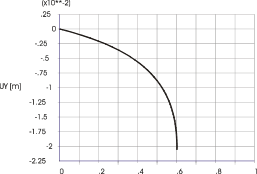
Ansys Toolbar>Quit>Save Geom+Loads, OK;
The linearized calculation (linearized buckling) determined the magnitude of the critical force ${{F}_{crit}}$= 266.6 N. The critical force value of the nonlinear solution can be obtained from the graph of increasing force versus the vertical displacement of the upper center line of the arc: The program determined the critical situation at ${{F}_{krit}}=0,6\cdot 300=180\text{ N}$. The difference in the critical force values is not negligible, and it should be noted that the linearized calculation provides the result on the "dangerous side".
In these stability examples we assumed a linear elastic material. For real problems with real materials it would be a very dangerous mistake to forget the possibility that the equivalent tensile stress at the most stressed points of the body can exceed the yield limit of the material before reaching the critical load in a purely geometrically nonlinear solution. Even with the least doubt about this, such a stability problem must be solved also as a the materially nonlinear problem.
[1] Puchner, O.: Strength of Materials II. Vydavateľstvo STU, Bratislava, 1997 (in Slovak)