Matrices of the nonlinear beam element (large displacements, large rotations, small deformations)
In Chapter Ch4, we dealt with a plane beam element for large displacements and rotations. We noted that for beams (beam finite elements) with a constant relative strain along their length, the formation of element matrices is relatively straightforward, as it is not necessary to express the displacement or strain of a general point on the beam. In such a case, the deformation is expressed in terms of the coordinates and displacements of the end points of the beam. It is also possible to introduce the assumption (approximation) that the cross-section of the beam and the modulus of elasticity remain constant during deformation, and to perform the integrals over the initial volume or the initial length of the beam. We have demonstrated this by developing matrices for a planar beam element suitable for solving problems involving large displacements and rotations and small deformations. We used Green’s deformation measure and, to determine the element matrices, we utilized the principle of minimum total energy of the bar. The choice of Green’s deformation simplified the formulation to such an extent that the elements of the element matrices could be expressed explicitly in terms of the element’s general parameters.
Building on the work [1] we now derive the fundamental matrices of such an element using vector calculus and the principle of virtual displacements. This is an elegant, albeit somewhat less intuitive, procedure by which the matrices of both planar and spatial elements can be derived simultaneously.
Vector of internal nodal forces in the element
Let us consider an arbitrary element of a planar bar structure (Fig.1) cut out immediately adjacent to the nodes, the length of which, in the initial (unloaded) position, is determined by the magnitude of the vector
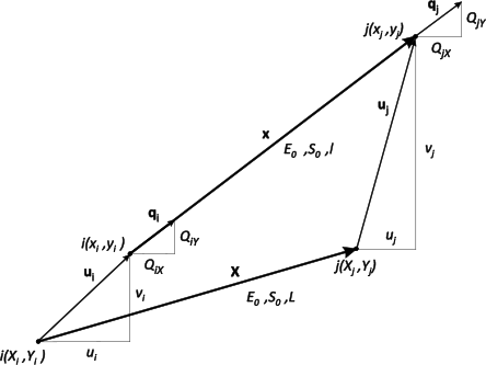
where
and the square of the bar’s length is
For the vector $\mathbf{x}$ , which specifies the length of the member after loading, the following applies
where
so the square of the length of the bar has changed under the effect of the load to
We can now express the deformation of the bar using any of the one-dimensional measures in use; for simplicity, we shall choose Green’s measure
whose variation is
The bar is cut out by an imaginary section from the system just past the nodes, and its equilibrium state after loading is ensured by the internal nodal forces ${{\mathbf{q}}_{i}}$ and ${{\mathbf{q}}_{j}}$ (which in this case behave as external end forces on the bar – see Fig.1), and the principle of virtual displacements applies to its equilibrium
Since we are dealing with a problem involving small deformations, it is possible to integrate in the along the initial length of the beam, L; and after substituting $\delta {{\varepsilon }_{G}}$ from , we obtain
Transposing this equation and rearranging gives
After choosing appropriate virtual displacements (unit and zero) and expressing the integrals, we obtain two equations
where$\mathbf{n}$ is the unit vector in the direction of the rod at its current (loaded) position. The axial force in the direction of the rod, using Green’s deformation, is thus
The distortion of the force N caused by the ratio${\ell }/{L}\;$ is negligibly small for problems involving small deformations
If, for a linearly elastic material, we choose a simple constitutive equation
then, for the internal nodal forces in the bar according to , the following applies
Substituting ${{\varepsilon }_{G}}$ and $\mathbf{x}$ would clearly demonstrate the nonlinear dependence of the components of these forces on the components of displacement.
It is true that in FEM, complete vectors (column matrices) of the element are used
where the nodal vectors are one-, two- or three-component, depending on whether the element is used in one-, two- or three-dimensional space. The relationships derived so far can also be applied to these vectors using the matrix
where $\mathbf{I}$ is the identity matrix of size 2×2 for a planar element and 3×3 for a three-dimensional element. Applying this matrix to (3), (7) and (15), we obtain
and finally the vector of internal nodal forces of the element expressed in terms of spatial (current) coordinates
and using the material (initial) coordinates
Tangential stiffness matrix of the element
The tangential stiffness matrix of the element is expressed as the relationship between the differential increment of the element’s displacement $d\mathbf{u}=d\left( {{\mathbf{u}}_{j}}-{{\mathbf{u}}_{i}} \right)$ and the differential increment of the vector of internal nodal forces $d\mathbf{q}$ . According (14) to and (15), we obtain
and for the derivative of N with respect to components of $\mathbf{u}$ with regard to (14) and (7), we obtain
Substituting this expression into (22) and (23), we obtain the result
where $\mathbf{K}_{akt}^{e}$ is the tangential matrix of the element expressed in terms of the element's spatial (current) coordinates (4), with the first matrix in this relation being called the material stiffness matrix and the second the geometric stiffness matrix.
The stiffness matrix of the element expressed in terms of the material (initial) coordinates is obtained by substituting (25) into (4)
It consists of a linear stiffness matrix
the stiffness matrix of the initial displacement
the stiffness matrix of the initial stress
The matrix $\mathbf{K}^{e}$ is used in the so-called total Lagrangian formulation and in the analysis of truss structures using FEM.
Total and updated Lagrangian formulation
In the numerical analysis of nonlinear problems using FEM, the external load is usually divided into parts and the problem is solved in several loading steps. This is either because the external load has a nonlinear behaviour, or because the iterative procedure is unable to converge under full loading in a single loading step. In the Lagrangian description of the nonlinear deformation of a body, two basic formulations are used in such cases to determine its deformation and stress state:
the total Lagrangian formulation (TLF)
the updated Lagrangian formulation (ULF)
In both formulations, the reference (known) configuration is used in the current loading step. In the TLF, all quantities (displacements, forces, stresses) are expressed in terms of the initial, fixed configuration, and the measures of deformation and stress are most commonly the Green–Lagrange deformation tensor and the second Piola–Kirchhoff stress. In ULF, the geometry from the previous loading step is adjusted in the current loading step, and this then serves as the reference configuration for the next loading step. Since, in ULF, the reference configuration is thus deformed, the measures of deformation and stress are logarithmic or Almansi deformation (Chapter 4) and Cauchy stress. Both calculation methods have their advantages and disadvantages, and the choice of formulation depends on the type of problem and the material model used.
Solving a nonlinear beam system using the total Lagrangian formulation
We shall illustrate the principle of the TLF using the example of a numerical solution to a simple geometrically nonlinear beam system with large displacements and rotations, but small deformations. For programming purposes, we shall first explicitly express the vector of internal nodal forces and the tangential matrix of a general element of a planar beam structure, which, in the unloaded state, is in the initial (reference) configuration defined by the coordinates of nodal points i and j (Fig. 2.1). Upon loading, the member moves to its current position, and we organise the displacement components of the nodal points resulting from this movement into a vector
If we define${{X}_{ji}}={{X}_{j}}-{{X}_{i}}$ ,${{Y}_{ji}}={{Y}_{j}}-{{Y}_{i}}$ ,${{u}_{ji}}={{u}_{j}}-{{u}_{i}}$ ,${{v}_{ji}}={{v}_{j}}-{{v}_{i}}$ , then the following holds for the squares of the lengths of the unloaded and loaded members:
From the change in the length of the beam, Green’s relative elongation of the beam at the current position can be expressed as
From , we obtain the vector of internal normal forces in the element
where $k_X = (X_{ji}+u_{ji})/L_e$, $k_Y = (Y_{ji}+v_{ji})/L_e$ and, given the small deformations, we have defined the stress in the member as $\sigma_G^e = E_e \varepsilon_G^e$.
The tangential matrix of the element and its components can be expressed from the relations to
where
In the TLF method, it is not necessary to extract the matrix of initial displacements from the element’s material matrix, and the following holds
Calculation of a truss system in the Mathematica software environment 7
Deriving the vector of internal nodal forces and the tangential matrix of the element already enables the creation of a nonlinear FEM programme for solving bodies composed of such elements. In the chosen programming environment, it is now merely a matter of algorithmisation and programming. In [2], we incorporated the element into the Fortran programme NELMKP; here, we shall use it to create a straightforward programme in the widely accessible Mathematica 5 environment. We take the basis of the programme, as well as the example, from [2], but we have modified the programme to handle multiple loading steps in order to demonstrate the total Lagrangian formulation.
Example 1
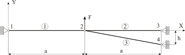
For the truss system shown in Fig. 2, determine the displacement of the point of application of force F and the magnitudes of the forces in the members, given a = 1000 mm and h = 50 mm. The material and cross-sections of the members are identical, with E = 200,000 MPa and S = 100 mm². The problem is to be solved—and the results presented—within a single computational cycle for force values of F = 2,000, 3,000, and 4,000 N. A Total Lagrangian formulation is to be used in the program.
Programme for solving the problem in Mathematica 7 and the calculated results