Plane truss element for large displacements and rotations
For trusses with a constant strain along their length, their FEM formulation is relatively simple because it is not necessary to express the displacement or deformation of a general point of the element. In such a case, the deformation can be expressed using the coordinates and displacements of the end points of an element. We will document this by creating matrices of a plane element suitable for solving problems with large displacements, rotations, and small deformations. We will use Green's strain for the deformation of the element and perform the integration of the internal energy of the element on the initial volume of the element. Such a formulation, in which the sought values are expressed using the initial configuration of the body (element), is called the total Lagrangian formulation. The choice of Green's strain simplifies the formulation to such an extent that all members of the basic matrices of the element can be expressed explicitly using the general parameters of the element.
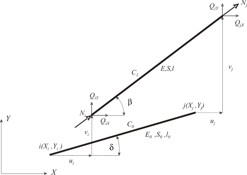
Let us consider an arbitrary element cut out close to the nodes by an imaginary section from a plane truss structure, which in the unloaded state is located in the reference position C0 (Fig. 4.1) determined by the coordinates of points i and j. After loading, the element reaches the actual position C1 and the components of the end point displacements that arise during this displacement are arranged in the vector
From the change in the length of the element, Green's strain at its current position can be expressed as follows:
If we introduce ${{X}_{ji}}={{X}_{j}}-{{X}_{i}}$, ${{Y}_{ji}}={{Y}_{j}}-{{Y}_{i}}$, ${{u}_{ji}}={{u}_{j}}-{{u}_{i}}$, ${{v}_{ji}}={{v}_{j}}-{{v}_{i}}$, then for the squares of lengths we have
and according for Green's strain of the element we get
The strain energy of the element is
The displacement of the element associated with its axial deformation will cause forces, the components of which are arranged into a vector
From the principle of minimum total potential energy of a body (we assume conservative external forces) for the equilibrium state of an element it follows (see Numerical (iterative) solution of nonlinear equations in femapplied.com)
The expression ${{{\partial {{\varepsilon }_{G}}}/{\partial \mathbf{u}}\;}_{e}}$ in (4.8) is a vector whose terms are obtained by successive differentiation (4.5) with respect to the components of vector (4.1)
where
${{k}_{X}}=\left( {{X}_{ji}}+{{u}_{ji}} \right)/{{l}_{0}}$ and ${{k}_{Y}}=\left( {{Y}_{ji}}+{{v}_{ji}} \right)/{{l}_{0}}$.
From the relation (4.8), (4.9) we can determine the components of the element's end forces corresponding to the specified displacements.
where the Green's force of the element is
and Green's stress is
The tangential stiffness matrix of the element is obtained by further differentiation of (4.8)
where $\mathbf{K}_{M}^{e}$ is the material stiffness matrix of the element (the linear part of $\mathbf{K}_{T}^{e}$).
The geometric stiffness matrix of the element (initial stress matrix) is obtained by (4.9) and (4.13), where each term of the vector $\mathbf{b}_{e}^{T}$ is derived with respect to all four terms of the vector ${{\mathbf{u}}_{e}}$
From the relations (4.8) and (4.13), we can express the vector ${{\mathbf{q}}_{e}}$ and tangential stiffness matrix of the element $\mathbf{K}_{T}^{e}$ for any measure of deformation when we replace the strain ${{\varepsilon }_{G}}$ in these relations with it. The formulation for the engineering strain with the correct constitutive relation ${{\sigma }_{ing}}={{E}_{0}}{{\varepsilon }_{ing}}$ is particularly interesting because the elastic modulus of the material is determined at this measure. Indeed, we lose the simplicity that the Green's strain of deformation of the member provides when deriving the vector of internal nodal forces of the element and the tangential stiffness matrix. Now it holds
and general vector terms
are also not simple. However, the Mathematica program performs the necessary derivatives without any problems, and determining the necessary element matrices is easy (Example 4.3).
A plane truss element can also be considered a simple body that has 4 degrees of freedom in the plane. If we remove three degrees of freedom from it, we obtain a statically determinate strength problem with one unknown, that is, the corresponding free component of the node displacement. The properties of the nodal force vector and tangential stiffness matrix of the element can be clearly demonstrated using example of such a body.
Example 4.1
Using the derived relations, the axial force, stress, and nodal force vector for the element given in Figure 4.2 are calculated in the case that it rotates by an angle of = 90° and stretches by 0.1 mm at node j under load.
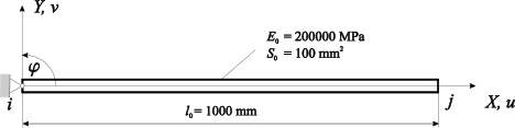
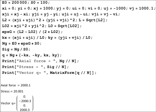
The position of the element is determined by the coordinates of nodal points ${{X}_{i}}={{Y}_{i}}={{Y}_{j}}=0,$ ${{X}_{j}}=1000\,mm$. The load was caused by displacements ${{u}_{i}}$= 0, ${{v}_{i}}$= 0, ${{u}_{j}}$= -1000, and ${{v}_{j}}$= 1000.1 mm. The solution to the problem and the results are shown in Fig. 4.3.
Example 4.2
Example 4.2 is solved using the engineering strain.
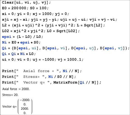
The solution is shown in Fig. 4.4. The force and stress results correspond to the experience with the engineering strain scale:
The physical meaning of the tangential stiffness matrix is the same as that in the linear problem: it expresses the stiffness of an element in a loaded computational model of a structure (body) in the equilibrium state. The larger the numerical value of its members, the stiffer the element, and vice versa. The tangential attribute only states that, unlike in the linear problem, it changes during loading depending on the changing displacements and rotations of the element. In the final (equilibrium) state, the material stiffness matrix represents the standard stiffness matrix known from the linear problem, although the iterative process must determine the position of the element relative to the global coordinate system. (There were no problems with this in the linear problem because the position of the loaded element was identified with the initial position.) This can be documented by introducing the allowed simplification $\text{l}\approx {{\text{l}}_{0}}$ for this element. According to Fig. 4.1, we can introduce the following equation:
${{k}_{X}}=\left( {{X}_{ji}}+{{u}_{ji}} \right)/{{l}_{0}}=\cos \beta $, ${{k}_{Y}}=\left( {{Y}_{ji}}+{{v}_{ji}} \right)/{{l}_{0}}=\sin \beta $
and the material matrix (4.14) of the element can be rewritten as
which is the standard stiffness matrix of a plane element at a given position relative to the global coordinate system. Therefore, the material matrix of a nonlinear element expresses the stiffness of the element resulting from its material and dimensional stiffness and its position in the loaded structure. It also follows from (4.19) that during the translational movement of the element, its stiffness matrix does not change.
In the linear calculation, we neglect the effect of displacements of nodal points on the material stiffness of the element, and in (4.19) holds (see Fig. 4.1)
${{k}_{X}}={{X}_{ji}}/{{l}_{0}}=\cos \delta $, ${{k}_{Y}}={{Y}_{ji}}/{{l}_{0}}=\sin \delta $
The geometric matrix of an element (4.15) affects the stiffness of the element depending on the stress acting on the element; therefore, it is often called the stress stiffness matrix. In our case, the size of the members was influenced by the size of the axial force and, therefore, by the axial stress of the element. This matrix plays an important role in the analysis of the loss of stability, effect of stress on bending stiffness, and change in the dynamic properties of the structure. We analyze its function using a beam nonlinear element in Beam instability and stress stiffening (femapplied.com).