Relations between displacement and deformation. Geometric equations
Small deformations
Consider a deformable body in a Cartesian coordinate system subjected to a static system of external forces. Since the body is constrained against rigid-body motion, these forces alter its initial configuration (geometry); the material points of the body move to new positions, i.e., the body deforms.
Assume that the displacement vector of the material points of the body is known (in the FEM, it is provided on finite elements in an approximate form)
where the continuous functions u, v, and w are the displacement components of a general point (x, y, z) in the directions of the coordinate axes. We seek the relationship between these functions and the functions that express the degree of deformation of the body at its points.
Let dx dy dz denote the differential (infinitesimal) volume element inside the unloaded body at a general point (x, y, z) (Fig. 1.1).
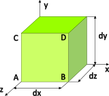
Due to the loading, the element is displaced in space and deformed. Owing to its very small dimensions, a simple strain mode associated with the definition of stress is considered: its linear dimensions change – it stretches or shortens in the directions of the coordinate axes – and theright angles between its faces are distorted.
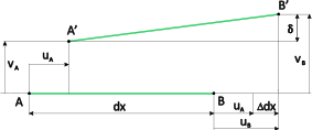
Consider two points, A and B, of the element located on an edge parallel to the x-axis and separated by dx (Fig. 1.2). As a result of the loading, the original positions of points A and B change. The line segment moves, changes its length, and rotates. For small deformations, the effect of rotation on the length of the segment is neglected, and the degree of deformation (strain) of the element in the x-direction is defined as the relative change in the x-distance between the points
i.e., the change in distance between the points $\Delta dx$divided by the original distance dx. Naturally, if the element translates as a rigid body in the x-direction, then ${{\varepsilon }_{x}}=0$. As can be seen, strain is a signed, dimensionless quantity (with the physical meaning of relative elongation or shortening).
The displacement ${{u}_{B}}$ can be determined from the expansion of the function u at point A into a truncated Taylor series. Owing to small deformations, only the first two terms are retained:
which represents the linearization of the function u at point A. Substituting (1.3) into (1.2) yields the relation for calculating the strain ${{\varepsilon }_{x}}$ at points of the body
It is the gradient of the function $u\left( x,y,z \right)$.
By an analogous analysis of the deformation of the element inin the y- and z-directions, we obtain
The functions ${{\varepsilon }_{x}}$ ,${{\varepsilon }_{y}}$ and ${{\varepsilon }_{z}}$, known as normal strains, cause a change in the volume of the element without violating the right angles between its faces, as they merely shift the parallel faces of the element by different amounts in the direction of their common normal.
However, the body load also causes so-called shear strains ${{\gamma }_{xy}}$, ${{\gamma }_{yz}}$, which disrupt the perpendicularity of the walls but do not alter the volume of the element. For example, if point C (Fig. 1.1) shifts in the direction of the x-axis relative to point A by a value $\Delta $, then according to Fig. 1.3
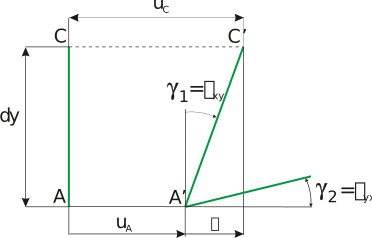
by re-using the shortened Taylor series for the ${{u}_{C}}$ we get
Thus, the vertical face of the element is inclined by an angle
Analogously, for the rotation of the horizontal face (Fig. 1.1) we have
and the shear deformation in the xy-plane (the total change in the right angle of the element in the xy-plane) is
By cyclic permutation of variables, we obtain the shear deformations in the other two planes
In summary, these linear shear components at the general point of the body can be expressed as a (pseudo) vector:
In matrix notation, the symmetric strain tensor considers the tensorial shear deformation ${{\varepsilon }_{ij}}={{\varepsilon }_{ji}}$ (Fig. 1.3) on each wall of the element (as a half value of the total shear deformation) and satisfies
where we get members from a simple index entry
In the displacement formulation of the strength problem, where the displacement field is the primary unknown, the strain relations (1.10) uniquely determine the strain field. The inverse problem arising in force formulations is more complex, because with six strain components, the three displacement components can be determined uniquely only if the constraints contained in the so-called compatibility equations are satisfied.
Large strains
The linear geometric relations between displacement and strain components (1.10), or (1.12), at material points of a deformed body are adequate for a large number of strength problems, since the important engineering materials (metals, concrete, wood, glass, etc.) allow only small strain values. For example, if a one-meter-long rod of constant cross-section is elongated by 1 mm, it results in a numerically small strain ${{\varepsilon }_{x}}=0,001$. However, such a strain in a steel rod induces a stress of approximately 200 MPa, which is at the yield limit of conventional steels and, for several less ductile materials, already beyond the strength limit.
On the other hand, there are a number of materials (e.g., industrial rubber, some plastics) and a number of technological processes (e.g., various types of metal forming) where the linear geometric equations are not applicable and more accurate relations must be used in simulation calculations. The derivation of these relations is not trivial; several methods and strain measures are employed, and their application in the FEM is also nontrivial. Here we present only the geometric derivation of the components of the Green-Lagrange strain tensor, which already provides some insight into nonlinear geometric relations. It should be noted, however, that the properties and applicability of each strain measure can be explained more clearly only together with its energetically conjugate stress measure.
Returning to Fig. 1.2, let us determine the change in length of the line connecting points A and B, taking into account also the effect of the different displacements of these points in the y-direction. We denote this difference by $\delta $ and, by approximating the function around A using the truncated Taylor series, we obtain
so
and the deformed length of the segment is expressed by the Pythagorean theorem
We introduce the relative deformation (denoted as in the case of small deformations)
The function of shape $\sqrt{1+x}$ can be decomposed into a series $1+x/2+{{x}^{2}}/8+...$ and the previous relationship after approximating the member with a square root by two series members is given by
Analogously, it can be shown that
It can be seen that when the strains are sufficiently small, the quadratic terms can be neglected and we obtainget the deformation components derived for the linear case.
The previous relations can be completed with analogous terms for the z-direction, and the independent components of the Green-Lagrange strain tensor can be written in vector form
or in concise index tensor notation
Remark 1: If a bar (rod, truss) with a length ${{\ell }_{0}}$ parallel to the x-axis at the end (located at the beginning of the coordinate system) is fixed and stretched by $\Delta \ell $ at the other end, its length will change to $\ell ={{\ell }_{0}}+\Delta \ell $ and the displacement function will be
According to relationship (1.4) valid for small deformations, the standard "engineering" strain of the bar is
From (1.13) we obtain the Green's strain
For small deformations (${{\varepsilon }_{ing}}<<1$) the difference between the two measures is negligible:
The Green-Lagrange strain tensor is independent of rigid-body translation and rigid-body rotation and is therefore frequently used in the FEM for problems involving small strains but large displacements and large rotations in the so-called corotational coordinate system.
Remark 2: Let's return to the figure from which we determined the components of the Green-Lagrange strain tensor:
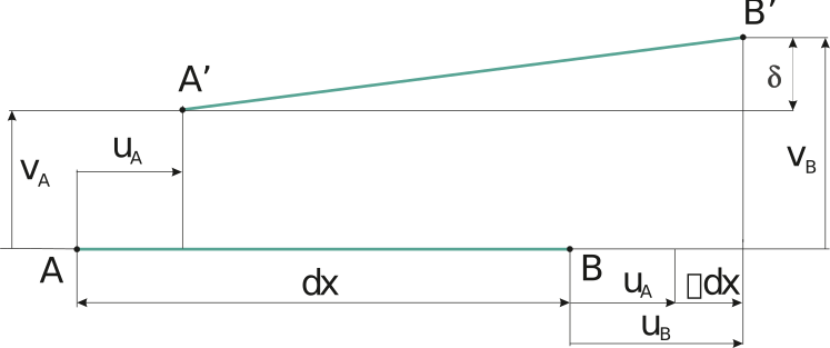
The Green-Lagrange strain is, as already mentioned, expressed by the ratio
It is an expression analogous to that for small deformations, but note that the direction of the segment A'B' and hence the direction is now different from the direction of AB, i.e., dx. The component has a direction identical to the direction into which the segment dx is rotated under loading. If in the next loading step the segment is only translated and rotated without changing the distance A'B', the magnitude of the strain does not change. The components of the Green-Lagrange strain follow the rotation of the element (material particle) in their direction, but their magnitude is independent of this rotation (and, of course, of rigid-body translation). This also applies to their energetically conjugate stress components – the second Piola-Kirchhoff stress.